Unit 1 – Exploring One-Variable Data

Individuals can be anything – people, animals, objects, etc.

Variables: any characteristics that changes between individuals - Categorical variables place an individuals into discrete groups or categories (e.g., ethnicity) - Quantitative variables can take numerical values (e.g., height)

Representing Categorical Variables

Tables:

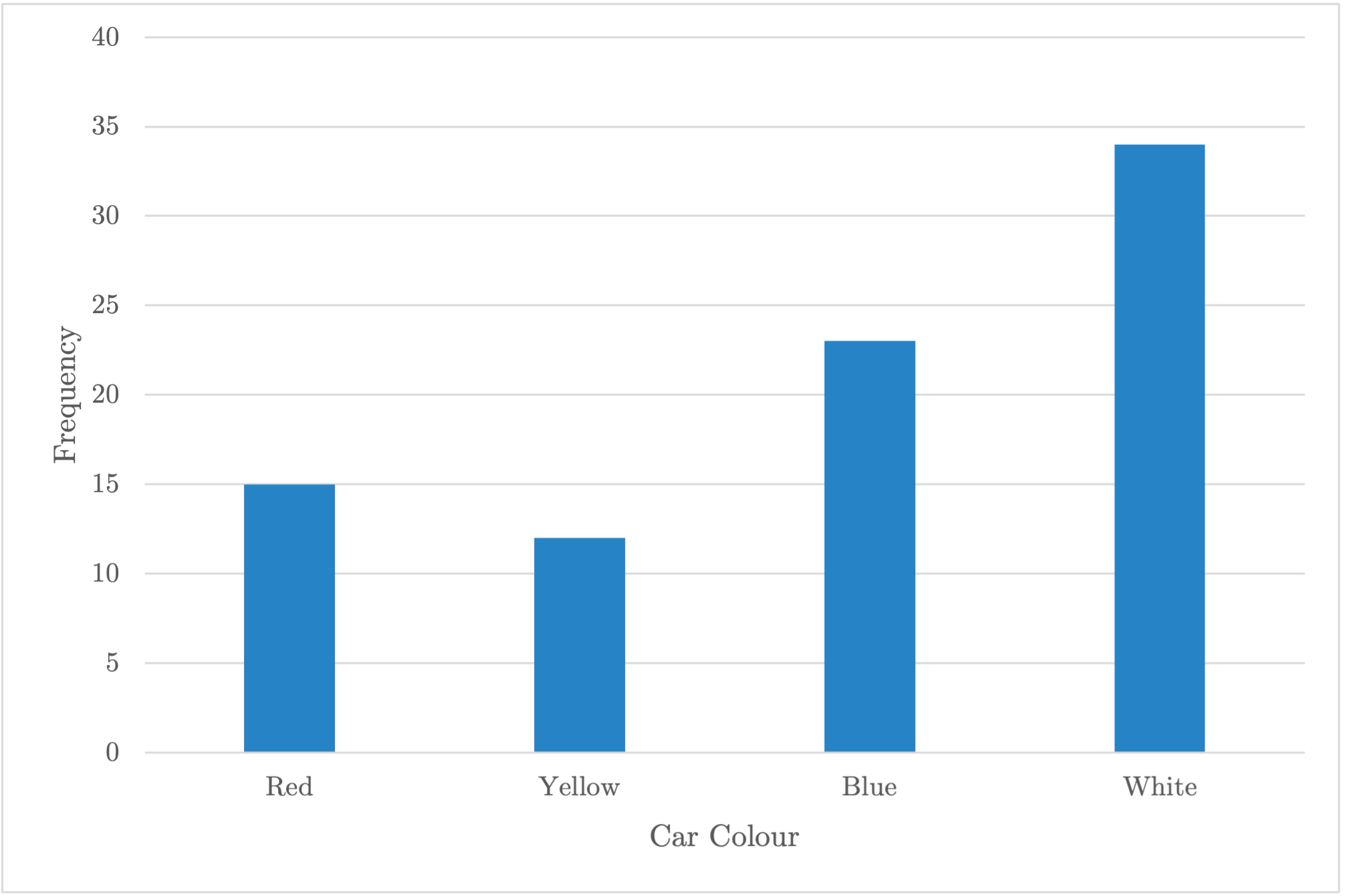
Car Colour	Frequency	Relative Frequency
Red	15	0.179
Yellow	12	0.143
Blue	23	0.274
White	34	0.405

Pie Charts or Bar Graphs:

Pie Chart	Bar Graph

Pie graphs show relative frequency. Bar graphs can show either frequency or relative frequency.

Representing Quantitative Variables

Quantitative variables may be either continuous or discrete. Bins are defined intervals which are equal in size, which are the quantitative equivalent to categories.

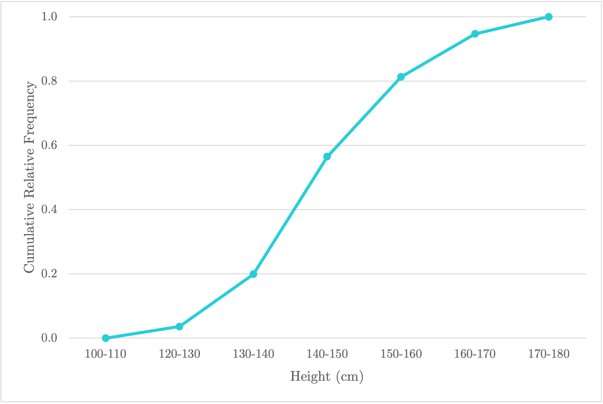
The four visualizations are dot plots, stem-and-leaf plots, histograms, and cumulative graphs.

Histogram	Cumulative Graph

The distribution of a quantitative variable is described in terms of:

• Shape: is the graph unimodal or bimodal? does it skew to one direction? are there any clusters or gaps?
• Centre: what is the (approximate) average?
• Spread: where are the majority of data located?
• Outliers/unusual features: are there any unusual points?

The above histogram can be described as:

Symetric and unimodal with a centre around 140cm. Heights are spread from 100 to 170cm, but little spread from where the majority are from 130 to 150cm.

Measures of Centre

The mean is sum of the values divided by the number of values

$$\overline{x}=\frac{\Sigma x_i}{n}$$

The mean is nonresistant. It can be influenced by outliers and skewness.

The median is the middle ordered value. When there an even number of values, it is the average of the middle two values.

The median is resistant. it is not influenced by outliers and skewness.

When data is symmetric, the mean is close to the median. When data is left-skewed, mean < median and vice-versa.

Measures of Position

Percentile: a value at the ${\text{K}}^{\text{th}}$ percentile will have $\text{K}\%$ of the data less than or equal to itself.

Quartile: a multiple of the $25^{\text{th}}$ percentile

• The median is at the $2^{\text{nd}}$ quartile or $50^{\text{th}}$ percentile
• The $1^{\text{st}}$ and $3^{\text{rd}}$ quartiles are the medians of the bottom and top halves

Measures of Spread

Range: max - min; easily influenced by outliers

Interquartile range (IQR): $Q_3-Q_1$; not influenced by outliers

Standard deviation (SD/$\sigma$): how far typical values are from the mean

$$s_x=\sqrt{\frac{\Sigma (x-\overline{x}{)}^2}{n-1}}$$

• Large SD: majority of data far from the mean
• Small SD: majority of data close to the mean

Outliers

Outliers can be determined in two ways:

Fence method: an outlier is a value less than $Q_1+1.5\cdot \text{IQR}$ or greater than $Q_3+1.5\cdot \text{IQR}$

2SD method: an outlier is a value $\pm 2\sigma$ from the mean

Transforming Data

Addition and subtraction affects centre and position but not spread.

Multiplication and division affects all measures.

Adding or removing data can have a major impact on nonresistant measures if outliers are present.

Box Plots

Normal Distribution

The normal distribution models populations. 68% fall within 1$\sigma$ of the mean $\mu$, 95% within $2\sigma$ of $\mu$, and 99.7% within 3$\sigma$ of $\mu$, however the distribution continues to $\pm \infty$.

Z-Score

The z-score measures how many standard deviations a value falls above or below the mean. It can be used to compare different data as it is a standardized measure.

$$\text{z-score}=\frac{x-\mu }{\sigma }$$

For example, a student with an IQ of 132 would have a z-score of

$$\frac{132-100}{15}=2.13$$

meaning they fall approximately 2.13 standard deviations above the mean.

Cumulative Distribution Function

The cumulative distribution function (CDF) of the normal distribution is the integral of the normal distribution, representing the percentage falling within the bounds of integration.

On the FX-CG50, the normal CDF can be accessed through the Run-Matrix or Statistics applications.

In Statistics: Dist > NORM > Ncd

• Set Data to Var

In Run-Matrix: OPTN > STAT > DIST > NORM > Ncd

• The NormCD() function takes the following arguments:
  • lower bound (use a large negative value to represent $-\infty$)
  • upper bound (use a large positive value to represent $+\infty$)
  • standard deviation ($\sigma$)
  • mean ($\mu$)

When calculating CDF using a z-score, $\sigma =1$ and $\mu =0$.

• $P(IQ<132)=P(Z<2.13)$

According to the normal CDF, a student with an IQ of 132 would fall at the $98.4^{\text{th}}$ percentile:

>>> NormCD(-100000, 132, 15, 100)
0.9835513

Conversely, only 1.64% of the population would have an IQ above 132:

Normal C.D
Data    :Variable
Lower   :132
Upper   :100000
σ       :15
μ       :100

Normal C.D
p    =0.01644869

Inverse CDF

The inverse normal CDF takes a percentile and returns the value or z-score at that percentile.

In Run-Matrix: OPTN > STAT > DIST > NORM > InvN

• InvNormCD takes the following arguments:
  • percentile
  • standard deviation ($\sigma$)
  • mean ($\mu$)

A person at the 80th percentile would have an IQ of 112.6:

>>> InvNormCD(0.80, 15, 100)
112.6243185

or a z-score of 0.84:

>>> InvNormCD(0.80, 1, 0)
0.8416212336

Standard Normal Tables

Standard normal tables return the integral of a normal probability density function from $-\infty$ to the z-score, which can be used to calculate the left NormCD manually.

To find the percentage at or below a z-score of 2.34:

We find the row 2.3 and column 0.03, returning 0.4904.