In macroeconomics, the aggregate supply/aggregate demand (AD/AS) model is used to establish equilibriums and study the effects of shifts in supply and demand.
- Keynesian theory focuses on the short run and aggregate demand
- Neoclassical theory focuses on the long run and aggregate supply
Say and Keynes’ Laws
Say’s law states that supply creates its own demand.
For every car bought, the salesman makes a commission which he then spends elsewhere, becoming another person’s income.
Neoclassical economists subscribe to Say’s law. The idea that supply creates demand is countered by the fact that recessions occur, but works better as a long-run approximation.
Keynes’ law states that demand creates its own supply.
Keynes’ works during the Great Depression argued that economies produce below their maximum potential due to a lack of demand, and thus incentive to produce. GDP is then determined by total demand, rather than what could be supplied.
The Keynesian perspective is countered by the idea that if governments stimulate demand through spending and policy, economies still face constraints to supply at some level. Keynes’ law is more effective in the short run.
The AD/AS Model
Potential GDP
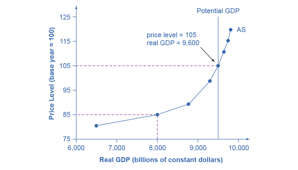
Aggregate supply is the output quantity (real GDP) produced and sold by firms. The AS curve shows the relation between real GDP (horizontal axis) and price level (vertical axis).
 |
|---|
| The AS curve models how the market responds to changes in final output price, meaning input prices such as labor and energy are assumed constant. Real GDP rises with the price level since firms have greater incentive to increase production. At low price levels, a small increase will lead to a large jump in GDP, since resources are underutilized and many people may be unemployed. Approaching the potential GDP, the level at which the economy is running at full speed, real GDP is less responsive since limits are being reached (the slope is far steeper). Potential GDP is also known as full-employment GDP, since the GDP reaches potential at natural unemployment levels. AS may cross potential GDP if people work overtime and machines are on overdrive. However, such production is only sustainable in the short run. |
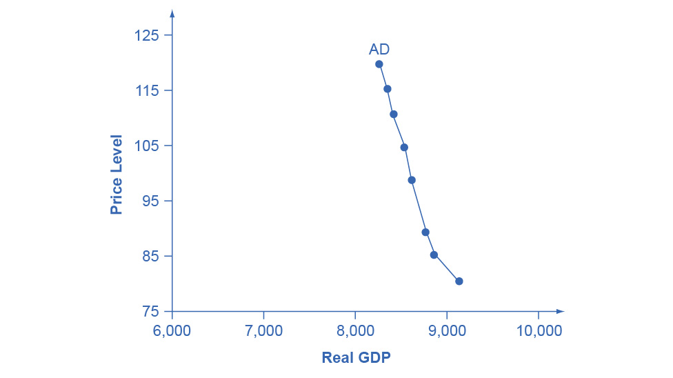
Aggregate demand is the total domestic spending (also real GDP) within an economy. AD is comprised of the components from GDP by demand, .
 |
|---|
| The wealth effect: As price level increases, buying power decreases. Consumers are less inclined to spend their money which is worth less due to inflation. The interest rate effect: As output prices rise, more money, and thus credit, will be needed. This increased demand increases rates, decreasing business investment and household borrowing. The foreign price effect: If the price of a nation’s domestic goods rises relative to other nations, exports will fall and more goods will be imported, reducing the export portion of GDP. AD has a steep curve, meaning there is little change in real GDP from changes in price level. |
Equilibrium
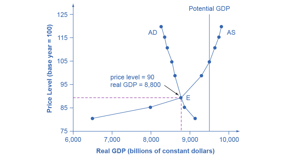
The AD/AS curves reach equilibrium at their intersection point.
When the price level is below equilibrium, firms are not incentivized to produce, but consumers want to purchase a lot. This triggers inflationary pressure, raising the price level until demand falls to to meet supply.
 |
|---|
| An equilibrium where AS is relatively flat means that GDP is below potential. Price levels are stable, but unemployment is higher. This economy could be in recession. An equilibrium where AS is steep means that GDP is near or at potential. Unemployment is low, but price levels are rising with inflationary pressure. |
Short and Long Run
The above AS curves are essentially short run aggregate supply (SRAS) curves. Firms can respond by adjusting supply and thus GDP to meet equilibrium in the short run.
However, supply will eventually reach a limit given enough time to make these adjustments. The potential GDP curve also represents long run aggregate supply (LRAS).
AS Shifts
 |
|---|
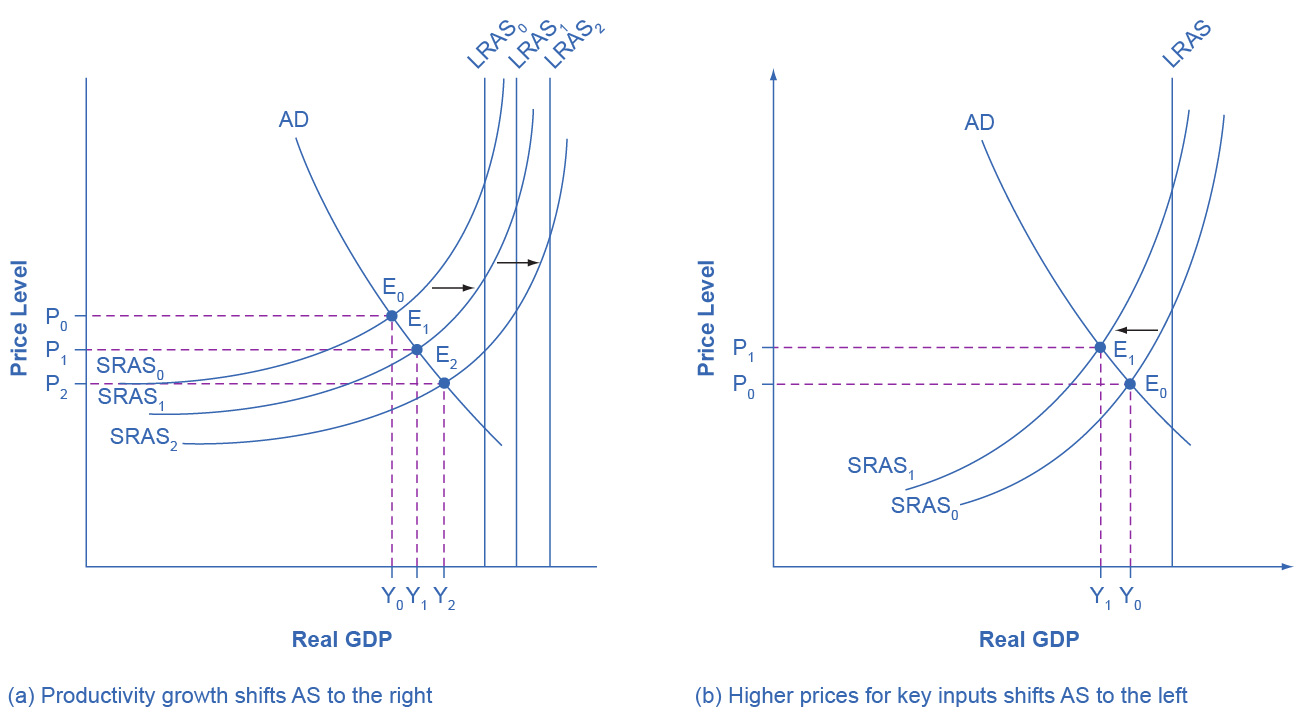
| The aggregate supply curve primarily shifts due to two factors: Productivity and Input Prices. |
| Increased productivity causes a right shift and vice versa. LRAS moves with productivity, since it is considered a limiting factor for real GDP. |
Decreased input prices causes a right shift and vice versa. These inputs include energy, wages, and imports. LRAS will not move with input prices.
Right shifts are positive, lowering price levels and unemployment while increasing GDP.
Left shifts are negative, increasing price levels and unemployment while decreasing GDP.
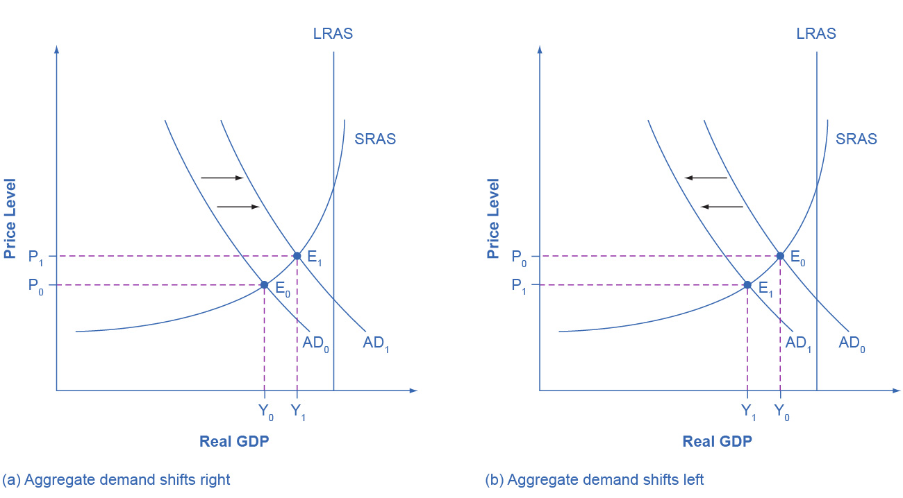
AD Shifts
Shifts in aggregate demand can be attributed to at least one of its components. For example, since imports is subtracted, aggregate demand decreases if imports increase. This is because less domestic production is demanded.
 |
|---|
| AD can shift left and right due to consumer and business behavior as well as government policy. |
| Right shifts increase real GDP in addition to price levels. They may be due to: |
- Increased confidence in the economy
- Increased government spending
- Decreased taxation
Left shifts decrease real GDP and price levels. They may be due to:
- Decreased confidence in the economy
- Decreased government spending
- Increased taxation
Growth
In the long run, AS will shift outward year-over-year, while equilibrium plays catch-up. Real GDP is close to potential during periods of growth, while the opposite is true during recession.
Unemployment
The natural rate of unemployment is one of the limiting factors of LRAS, which is reflected through the AD/AS model. Countries with higher natural unemployment could see lower potential.
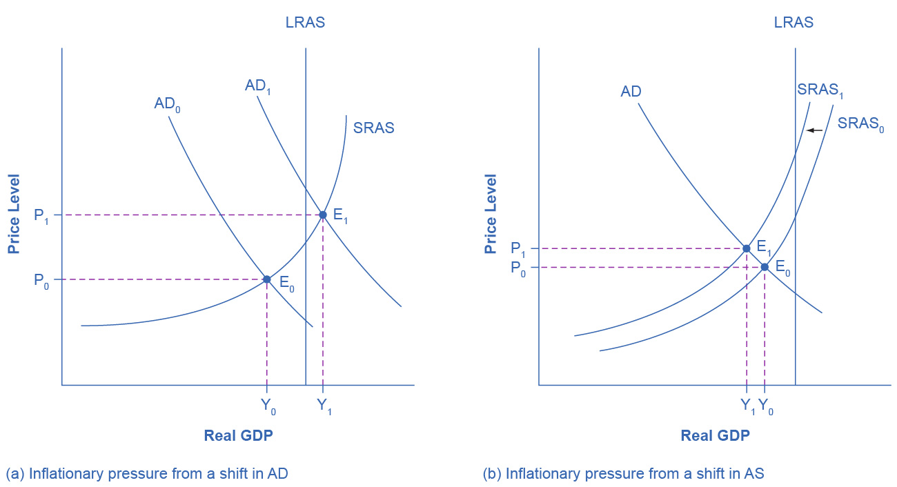
Inflationary Pressure
Inflation tends to be greater during periods of growth, while recessions could lead to deflation.
 |
|---|
| Right shifts in AD near LRAS can trigger inflation by entering a steeper portion of the SRAS. The economy may be operating at capacity. Left shifts in AS can trigger inflation as well. Higher input prices can passed along to the buyer. |
We only model one-time shifts. Sustained inflation can be due to government actions to cause left AD shift and/or increasing prices, wages, and rates in response to predicted inflation (which can require government intervention).
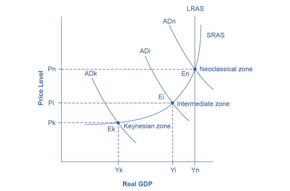
AD/AS Zones
 |
|---|
| The Keynesian zone is the shallow portion of the SRAS curve. Inflation is low, GDP is below potential, and unemployment is high. The Neoclassical zone is the steep portion of the SRAS curve. AD shifts cause high inflation, while AS shifts are needed to grow GDP. The unemployment cycle is at its lowest. The intermediate zone falls in between. Unemployment has an inverse relation with inflation and GDP. |